
Combining Data in Cells
3 ways to combine information from multiple cells into one.


Don’t forget to download the sample data at the end of the lesson so you can practice along!
One of the most important skills in Excel is understanding how to combine elements from multiple cells into one. This is because we can’t always predict how we will receive the data we want. It is quite often that we want to combine our data to create unique codes such as a phone number, place a first & last name into a single cell, or create a custom header to our sheet that updates based on new information.
Luckily for us Excel offers 3 simple methods that we can use to help us with this challenge. In todays lesson we will explore each of these and learn how to use them step by step.
Using Ampersand AKA “&”
The Ampersand or “&” operator joins the contents of multiple cells together. It works with both values and text. The result of joining these cells using “&” is always formatted as text. Lets look at an example:
In this case we have an Area Code + Phone Number. However they are broken up into 2 separate cells. Ideally we want them in one combined cell. Here is how we can use “&” to fix that.
Step 1: Identify the cells that you want to combine. In this case it will be data in Column A combined with data in Column B into Column C.

Step 2: Type in a formula that places an “&” between the two cells. In this case it will look like this:

Step 3: Fill down the formula to perform the task on the rest of the data.

=CONCAT()
=CONCAT is perhaps the most well known and popular way to combine data inside of cells. It removes the need to use the “&”. While many will forever debate the value of one over the other, it is good to understand how to use both. Then you can decide for yourself which one you prefer. I personally have used a mix of both in the past, depending upon the situation.
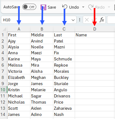
In this example we will use =CONCAT to combine first, middle, & last names into one cell with a space in between.
Step 1: Identify the cells you want to combine. In this case we want to combine Columns A, B, & C into Column D. We also want to add a space in between each part of the name.
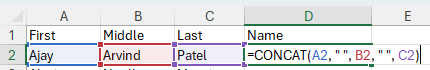
Step 2: Enter in the =CONCAT formula. Here is its syntax:
=CONCAT(text1, [text2], …)
text1 is required. This is the first item to join.
[text2], … are optional. These are additional text items that you want to join, up to 253 items.
In this case the final syntax would look like this:
Step 3: Fill down to complete the task with the rest of the data:

=TEXTJOIN()
=TEXTJOIN() is the newest of the 3 methods inside of Excel. It takes joining cells to another level of simplicity. What makes it so distinct is the ability to specify the cells you want to combine in an array, and then include a delimiter of your choice (i.e a space, dash, comma, etc.) With =TEXTJOIN you can also ignore or include empty cells within the range. This means you don’t have to go back and add or remove empty cells because of this.
Lets start with the syntax for =TEXTJOIN():
=TEXTJOIN(delimiter, ignore_empty, text1, [text2], ...)
Where:
delimiter: This is a required field. Here, you define the character (or characters) that you want to use to separate each of the text items that are being joined. This can be a comma, space, dash, or any other delimiter you need.
ignore_empty: This is also a required field. You will enter TRUE if you want the function to skip over any empty cells in your range or FALSE if you want the function to include empty cells in your range.
text1, [text2], ...: These are the cells, ranges, or strings that you want to join together.
text1 is required. This is the first item to join.
[text2], … are optional. These are additional items that you want to join, up to 252 items.
Let’s take a look at a simple example:
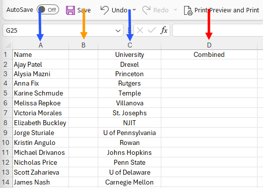
Step 1: Identify the cells you want to combine. In this case we want to combine an individuals name with their University. We want them separated by the dash, and we want to IGNORE the blank column between them.
Step 2: Utilize the =TEXTJOIN formula in the cell where you want to see your results. Here is what it looks like in this example:

Step 3: Fill down to apply to the rest of your list.

=TEXTJOIN() makes takes this important task and helps simplify it tremendously!
Thanks for reading this lesson on joining the contents of several cells. Make sure that you practice using these features. This is easy to do - just download the sample data set right here: