


TED #029: Splitting Up Data In Cells
Using Text-to-Columns to split up data from a single cell into multiple cells.


Don’t forget to download the sample data at the end of the lesson so you can practice along!
A few weeks ago we reviewed an important skill - combining data in cells. This particular concept is of massive importance. Being able to do the reverse, split up data, is also of great importance. Many times when we download data from a CRM, ERP, or whatever the source - it comes to us with multiple bits of information in a single cell.
Luckily for us Excel offers a very easy way to do this. In todays lesson we will explore a very popular and very legacy tool: Text-to-Columns.
Introducing Text-to-Columns
This particular feature has been around quite some time with Excel. It is very popular for cleaning up data, particularly from files knowns as .CSV or Commas Separated Values. However it offers a TON of options when it comes to splitting up data. You don’t have to have data separated only by commas. Any delimiter will do. You can also ask it to split up data based on a specific width as well. Lets look at an example.
Here is some data we recently downloaded from a payroll system. It has some basic employee info as well as pay info.
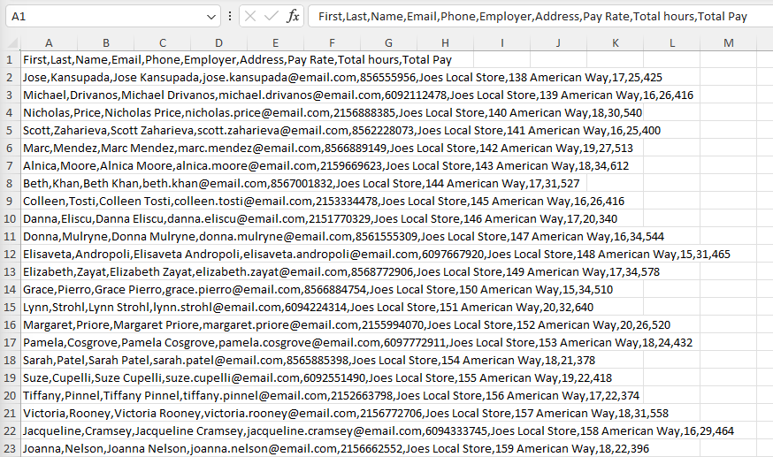
A couple of things to observe here.
The data is in a single cell. We can tell this simply by looking at the formula bar.
Each “piece” of data is separated by a comma.
There are many lines that are in this same pattern.
Note: in this example we show 23 lines. In my experience this can be several thousand.
Step 1: Now that we identified the key elements above we want to highlight the cells in which the data resides. In this case we would select the cells in Column A.

Step 2: In the menu go to Data>Text-to-Columns

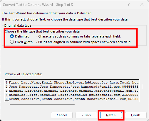
Step 3: The “Convert Text to Columns Wizard” opens up. This wizard will guide you step by step on how to convert your data. The first question - Delimited or Fixed Width. In this case you will want to choose Delimited since we know a delimiter (the comma) is what separates each value in the cell. Then click Next.
Step 4: The wizard will offer a few options for your delimiter. As you can see you aren’t just limited to commas. Excel recognize a host of delimiters, and you can pick more than one.

It even offers you the option to enter your own. I have used this a few times.

Once you select your chosen delimiter(s), the Data Preview section will give you an idea of how your data will be separated. Click Next once your satisfied with the preview.

Step 5: In this final step you will get the chance to add in some formatting and omit columns that are not relevant to what you need.
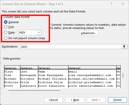
Click on each column and adjust as necessary. In our case we want to remove the column that has the combined first and last name. Here is how it looks:

When you’re done with each column, click Finish. The Text-to-Columns Wizard will now separate, remove, and format your data exactly as your requested.
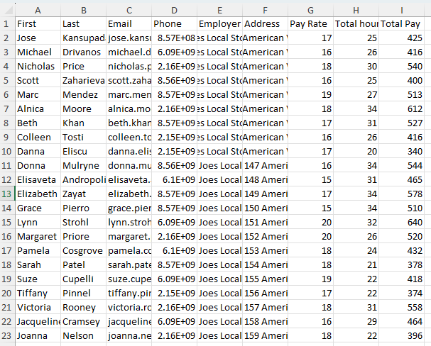
Step 6: Add in some additional formatting as needed and your data has turned from a hot mess into a a nicely organized data set that you can easily work with.

Thanks for reading this lesson on using Text-to-Columns to split up data from one cell into multiple cells. Make sure that you practice using this awesome feature. This is easy to do - just download the sample data set right here:
Apply what you have learned and it will stay with you much longer.
There are a few other ways I can help you master Excel:
Do you have any burning questions about Excel that you want answered? Send your question to ajay@theexceldojo.com. I will address it in a future newsletter.
Do you or your organization need a little spreadsheet help? Book a 1 on 1 with me here.
Want to learn more Excel Shortcuts? I have created something special (and free) for you: The Best Damn Excel Shortcut Sheet
Til next time ✌️
-Ajay
The Excel Ninja 🥷
PS - If you like these lessons please share with a friend or two...