


TED# 032: A Deep Dive into XLOOKUP - Part 3
Breaking down one of Excel’s most versatile and useful functions.


Don’t forget to download the sample data at the end of the newsletter so you can practice along!
Welcome back! This will be our 3rd installment in this series where we focus on XLOOKUP. To wrap things up we are going to cover 2 more topics: [search_mode] and two-way lookups. Before we do that, let’s do a quick review of the syntax so we can get right back up to speed.
Revisiting the syntax
Let’s review the syntax for XLOOKUP quickly:
=XLOOKUP(lookup_value, lookup_array, return_array, [if_not_found], [match_mode], [search_mode])
lookup_value: This is the value you want to search for. It can be a single cell OR an array.
lookup_array: Lookup array are the range of cells that will contain the value you want to lookup.
return_array: This range of cells will have the corresponding information that you want to return.
[if_not_found]: An optional argument that specifies what value you want to return if lookup_value is not found in search_range. The default is to return #N/A.
[match_mode]: Determines how Excel should match the lookup_value.
[search_mode]: Determines the direction of the search.
[search_mode]
Search mode is an element of the XLOOKUP function that allows you to determine the direction of the search. Here are the arguments that you can enter inside the [search_mode] element:
1 or omitted: Search first-to-last (default).
-1: Search last-to-first (useful for retrieving the last occurrence).
2: Binary search (sorted ascending).
-2: Binary search (sorted descending).
As we always do, let’s jump into an example where we will use search mode.
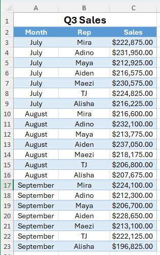
Here we have a list of sales reps. We want to find the very last entry for Maya since that will give us her September Sales number.
Step 1: Enter XLOOKUP and the following elements:
lookup_value: E3 (I have entered the rep name in this cell)
lookup_array: B3:B23
return_array: C3:C23
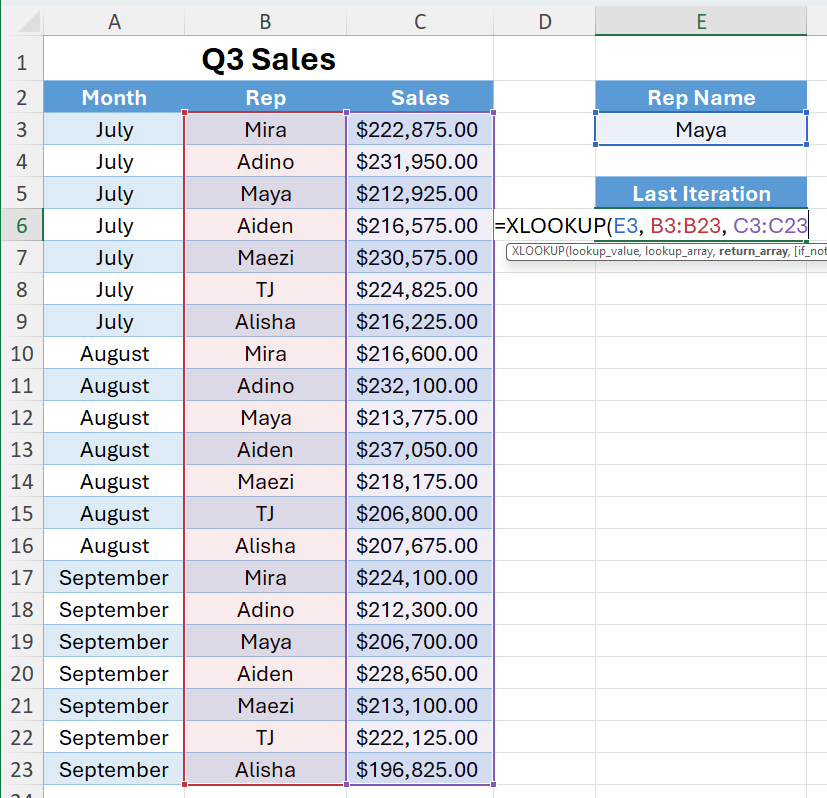
Step 2: Skip [if_not_found].
Step 3: Skip [match_mode].
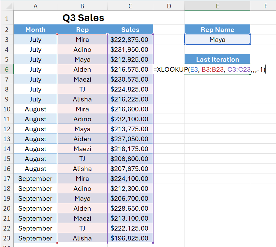
Step 4: For [search_mode] we will enter 1 of the 4 options listed. In this case we will select -1. This is used for searching last to first (bottom up) in the array.
Here is what it will look like:
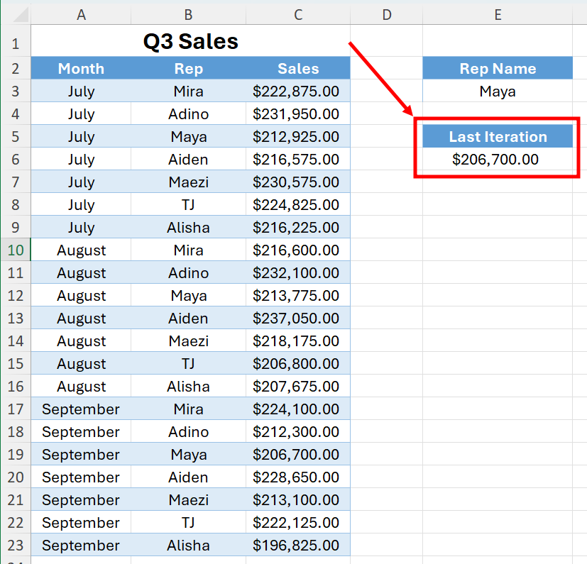
XLOOKUP will return the last iteration of Maya’s sales data in the table!
Two-way lookups
The search mode is a great element in the XLOOKUP formulas. However, what if we wanted to look up a the Sales total for a Rep based on the Month? This would be a two-way lookup. Let’s take the same data but arrange it a bit differently:

Step 1: Enter XLOOKUP and the following elements:
lookup_value: F6 (I have entered the rep name in this cell)
lookup_array: B2:D2

Now here is where things get exciting….
return_array: XLOOKUP
Now inside of this XLOOKUP enter the following elements:
lookup_value: F3 (I have entered the month into this cell)
lookup_array: A3:A9
return_array: B3:D9
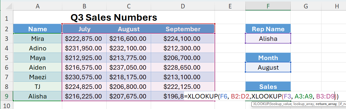
Voila! You now have a two-way lookup setup. Here is the result:

And here it is in action:
Thanks for taking the time to read this newsletter. XLOOKUP is a great formula to know and understand for users of all levels. I hope this series was able to open your eyes to it’s many applications!
Make sure you practice what we have covered today. Here is a link to the sample data so that you can follow along.
When you’re ready, there are a few other ways I can help you master Excel:
Do you have any burning questions about Excel that you want answered? Send your question to ajay@theexceldojo.com. I will address it in a future newsletter.
Do you or your organization need a little spreadsheet help? Book a 1 on 1 with me here.
Til next time ✌️
-Ajay
The Excel Ninja 🥷
PS - If you found this newsletter informative please share with a friend or two...