


TED #035: Creating Numbered Sequences in Excel - Part 3
A deep dive into Excel's =SEQUENCE Data Array Function


Welcome back everybody! This week we are going to dive into the last part of our series on creating numbered sequences in Excel. I decided to extend the series by 1 because I felt like the final topic needed it’s own time devoted to it. It is a Data Array Function known as =SEQUENCE().
The syntax
Before we dive into some examples let’s take a deeper look at how this particular function is structured.
=SEQUENCE(rows, [columns], [start], [step])
Here's a simple breakdown of each element:
rows (required): This is the number of rows you want in your sequence.
columns (optional): Here you decide how many columns you'd like your sequence to spread across. If you don't specify this, it defaults to one column.
start (optional): This is where your sequence begins. If you don't specify a start number, it will automatically kick off at 1.
step (optional): This is the increment between each number in your sequence. No input here will just default to an increase by 1 each time.
As you can see the syntax and elements for =SEQUENCE() are very straight forward.
A simple application
Let’s look at the most basic application. Creating a sequence of numbers from 1-20. Simply enter the following into a cell:
=SEQUENCE(20)
That’s it! Excel will “spill” the results into the cells as appropriate.
Going deeper with =SEQUENCE()
With 4 elements in the syntax there is plenty of room to explore. Let’s add one more element to the syntax. We will input the following:
=SEQUENCE(6,5).
We are asking the Excel to create a sequence of numbers 6 rows x 5 columns. Essentially Excel will be building a simple data array for us. Here are the results:
Let’s take it one more step - this time we will use all 4 arguments. We will keep the first 2, but we will start the series at 3 and increase by steps of 7. We will input the following:
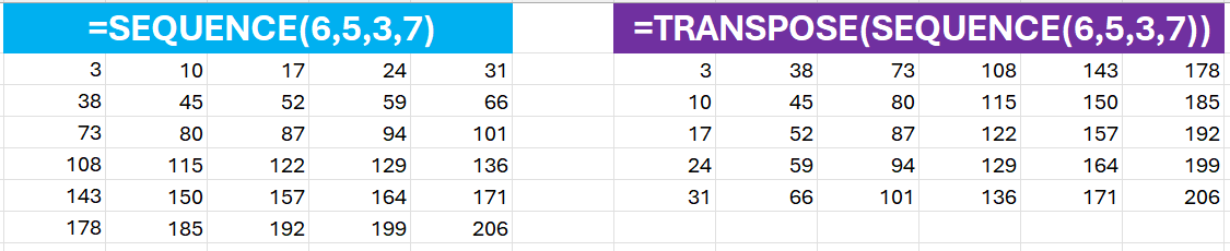
=SEQUENCE(6,5,3,7)
Nesting with other functions
Now you have seen what this formula can do just on it’s own. However the best parts are still to come. When combined with other functions we can really start to create some cool results using =SEQUENCE. Let’s take a look at a few examples.
Transpose
In the examples above you will notice that in the arrays created, Excel filled in the numbers by filling in each row from left to right. Once it hit its max number of columns it then moved down a row.
The problem is then evident - what if we want to fill in each column first from top to bottom? The move to the next column on the right? The solution is simple - we will simply nest our =SEQUENCE function with the =TRANSPOSE() function. Here is the syntax:
=TRANSPOSE(SEQUENCE(6,5,3,7))
We can see side by side how the two arrays are different:
Workday calendar
Creating a custom calendar in Excel used to be a pain. But it was worth it because of the versatility it offered us! By nesting =SEQUENCE() with =WORKDAY() we can create a simple M-F calendar that can make our life easy. Here is the syntax that makes it happen:
=WORKDAY(AC1-1,SEQUENCE(4,5))
In this case cell AC1 is the location of the start date. This is the first element in the =WORKDAY() function. We subtract 1 from it in order to make the =WORKDAY() start the sequence correctly in our calendar.
Random sequence between two numbers.
Our first instinct here is “why can’t I use =RANDBETWEEN()?” And that is a great question. The answer is simple - we only want 1 instance of each number. For example, lets say we would like each number between 1-10 to appear in a list in random order? To do this we nest 3 Excel functions. we will place =SEQUENCE() & =RANDARRAY inside of the =SORTBY() function. Here is what the syntax will look like:
=SORTBY(SEQUENCE(10), RANDARRAY(10))
Auto-labeling lines of data as they appear
I think I make use of this particular application the most. Being an engineer I like lists. For example - I create carousels for my content. When I storyboard them in Excel I like to have each slide numbered so I can match each slide with an image. This helps to keep things organized. I like for my list to say “Slide #1, Slide #2, etc.
Here is how I make that happen:
="Slide #"& SEQUENCE(COUNTA(AI:AI)-1)
In the example below observe how every time time a new description is added, a label for each row is added as well.
The reason why I subtract 1 in the COUNTA nested function is because I have to account for the Description heading.
Thanks for reading the final part of this series. I am really hopeful that you gained some good value here. The =SEQUENCE() function is so simple yet so versatile and important. By mastering it you can really simplify so many tasks in your daily life.
To help you with that I encourage you to make sure you practice what we have covered today. Here is a link to the sample data so that you can follow along:
When you’re ready, there are a few other ways I can help you master Excel:
Do you have any burning questions about Excel that you want answered? Send your question to ajay@theexceldojo.com. I will address it in a future newsletter.
Do you or your organization need a little spreadsheet help? Book a 1 on 1 with me here.
Be sure to follow me on your favorite social media platforms!
Til next time ✌️
-Ajay
The Excel Ninja 🥷
PS - If you found this newsletter informative please share with a friend or two...