


TED# 036: Exploring Dynamic Array Functions in Excel
Part 1: =UNIQUE()


I can remember the days when my excel sheets were packed with endless nested functions, and long macros.
While I was able to get pretty good at using excel in this way, the truth is that it made Excel so tedious to use for so many folks. It added to the intimidation factor for novice users. However the good folks at Microsoft recognized this issue and created Dynamic Array Functions (DAF’s).
Before Excel 2019 and Microsoft 365, when we used a function in Excel, it typically returned a single value in a single cell. We all learned how to use the fill formulas to help us return the answers across an array of variables. Or created massive Index-Match nestings needed to design 2 way lookups. I could go on & on…it was definitely tough!
What makes DAF’s so unique is that when these functions calculate multiple results, they "spill" them onto the worksheet into a range of cells. And the nature of the functions wrap what used to be complex nested functions into something simple.
Think of it like this - imagine you are making a fruit smoothie. The old method in Excel basically required you to blend each fruit individually. Then combine them. With DAF’s, we can throw all the fruit in the blender and get to work. It’s all about efficiency.
In this series I will do a deep dive into DAF’s every Excel user should know. This week we are going to dive into =UNIQUE.
A deeper dive into =UNIQUE:
Dealing with duplicates? This function extracts unique values, making data cleanup a breeze. Let’s dive into the syntax:
=UNIQUE(array, [by_col], [exactly_once])
array: The range of data from which you want to extract unique values.
by_col (optional): TRUE to return unique columns, FALSE to return unique rows. Default is FALSE.
exactly_once (optional): TRUE to return values that appear only once, FALSE (default) to return all unique values regardless of how often they appear.
Example:
Let’s take this set of Sales Reps.
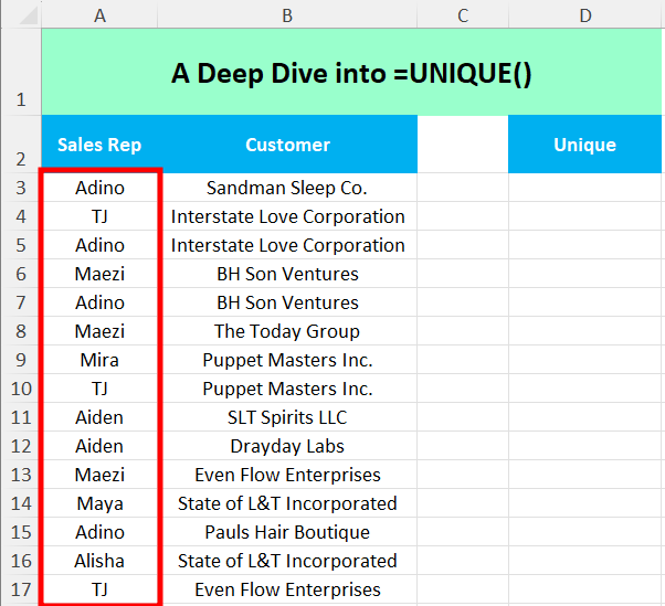
There are multiple reps but repeated many times. If we want to see a list of each name listed we would enter the following:
=UNIQUE(A3:A17)
What if we want just the names listed once?
There is nothing more unique than a single entry in a long list. Great news, =UNIQUE() can help us with that. Lets take that same list, this time we will use the following syntax:
=UNIQUE(A3:A17,,TRUE)
=UNIQUE() Works across rows also…
Let’s take the same data, but this time it exists in a single row vs column:
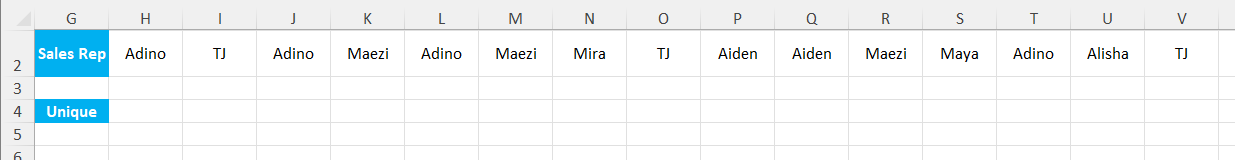
If we put in unique and highlight the row, we don’t get exactly what we were looking for….
This is where the second element of the syntax helps us. In this case we enter the following:
=UNIQUE(H2:V2, TRUE)
This elements indicates to Excel to find unique values across columns, which is how multiple values are listed in a single row.
Thanks for reading this newsletter. I am really hopeful that you gained some good value here. DAF’s are a major game changer in Excel, and this is just the start. They save you time, energy, and a lot of aggravation. By mastering them you can really simplify so many tasks in your daily life.
To help you with that I encourage you to make sure you practice what we have covered today. Here is a link to the sample data so that you can follow along:
When you’re ready, there are a few other ways I can help you master Excel:
Do you have any burning questions about Excel that you want answered? Send your question to ajay@theexceldojo.com. I will address it in a future newsletter.
Do you or your organization need a little spreadsheet help? Book a 1 on 1 with me here.
Be sure to follow me on your favorite social media platforms!
Til next time ✌️
-Ajay
The Excel Ninja 🥷
PS - If you found this newsletter informative please share with a friend or two...