
TED# 037: SORT & SORTBY
A must know function that helps us organize our data.


How often do you get asked to take the data you have and sort it? For me - constantly. I am willing to bet it’s the same for you. Sorting data is a huge benefit to using a spreadsheet program like Excel. Viewing information either chronologically, alphabetically, numerically, etc. is a concept that predates any spreadsheet software out there. This is why one of the most basic features of spreadsheets from the beginning was the ability to sort data. Excel is no exemption. It did a good job of this - but over time as with anything the needs of sorting became more complex. A new way was needed. Enter the focus of todays topic - SORT & SORTBY.
=SORT()
Lets start off pretty basic. The =SORT() function arranges your data in a specific order. You have two options - ascending or descending. Lets dive into the syntax:
=SORT(array, [sort_index], [sort_order], [by_col])
array: The range of cells you want to sort.
sort_index: Which column or row you'd like to sort by. (Default is 1)
sort_order: 1 for ascending (default) and -1 for descending.
by_col: If TRUE, it sorts by column instead of row.
Now let’s take a look at a simple example. Here we have a list of reps & their sales volume for the month.
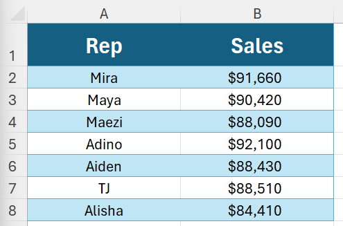
In the first scenario lets sort them alphabetically by name of the rep. We enter the following syntax:
=SORT(A2:B8,1,1)
Next, lets do the same but sort the data by sales, highest to lowest. Here is the syntax:
=SORT(A2:B8,2,-1)
=SORTBY()
=SORT() is pretty straight forward & simple. But what if we want to sort an array based on the values of a 3rd column? This is where =SORTBY() takes things to another level. Here is how the syntax breaks down:
=SORTBY(array, by_array1, [sort_order1], [by_array2], [sort_order2], ...)
array: The range of cells you want to sort.
by_array1: The first range of cells to sort by.
sort_order1: 1 for ascending and -1 for descending. (And so on for by_array2, sort_order2, etc.)
Back to our example - but this time we have added a 3rd column, Service Rating.

This time we would like to sort columns A&B by column C (lowest to highest). Here is how we do it:
Enter: =SORTBY(A2:C8, C2:C8, 1)
Here is where it gets really cool. Lets change up the service rating of TJ (Cell C7) and see what happens.
The list is automatically updated!
Nested with =UNIQUE
=SORT() & =SORTBY() are powerful functions especially once they are nested with other great functions. For example you could use the =UNIQUE() function to grab individual occurrences in a list and nest it inside of the =SORT() function to arrange them alphabetically! Here is another example. Lets look at this list of companies:
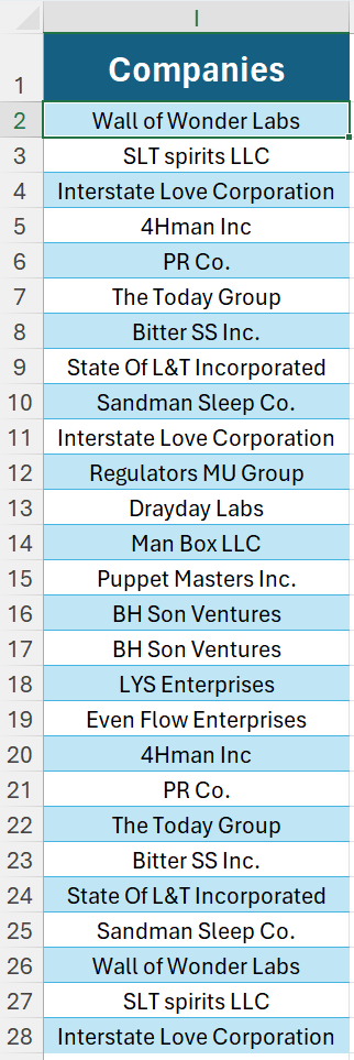
Now lets create a new list, but this time with only one occurrence of each company AND in alphabetical order. Here is our syntax:
=SORT(UNIQUE(I2:I28))
Thanks for reading this newsletter. SORT & SORTBY are two incredible functions that can really make your Excel files come to life. But as always you have to make sure that you practice them! To help you with that I encourage you to make sure you practice what we have covered today. Here is a link to the sample data so that you can follow along:
When you’re ready, there are a few other ways I can help you master Excel:
Do you have any burning questions about Excel that you want answered? Send your question to ajay@theexceldojo.com. I will address it in a future newsletter.
Do you or your organization need a little spreadsheet help? Book a 1 on 1 with me here.
Be sure to follow me on your favorite social media platforms!
Til next time ✌️
-Ajay
The Excel Ninja 🥷
PS - If you found this newsletter informative please share with a friend or two...