TED #038: =FILTER() Your Way to Efficiency
Discover how the =FILTER() function can streamline your data analysis, making spreadsheet tasks simpler than ever.
In today's newsletter, we're diving deep into Excel's dynamic array functions with a special focus on our superstar for the day - the FILTER function. A game-changer in spreadsheet data management, these functions, particularly the FILTER function, have revolutionized the way professionals handle, analyze, and present data. Whether you're a newcomer or an experienced Excel user, understanding the nuances of these functions is pivotal in today's data-driven environments. Let's get started and explore the mechanics and applications of the FILTER function.
Let’s get started…
The basics of =FILTER()
This formula allows you to filter data based on specific criteria. The syntax for the filter formula is:
=FILTER(array, include, [if_empty])
Where
array: The range of data that you want to filter. This can be a cell range, a named range, or an array.
include: The conditions that you want to include in the filter. This can be a single condition, a range of conditions, or an array of conditions.
if_empty (optional): The value to return if the filter returns no results. This can be any value, such as an empty string, a number, or an error message.
Lets look at a simple example:
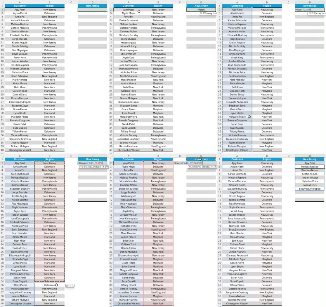
Here we have a list of customers and the region where they exist:
Lets create a filter to look at all the customers only in New Jersey. Here is the syntax:
=FILTER(A2:A40, B2:B40=D1)
As you can see, all of the customers in New Jersey are now in a clean list.
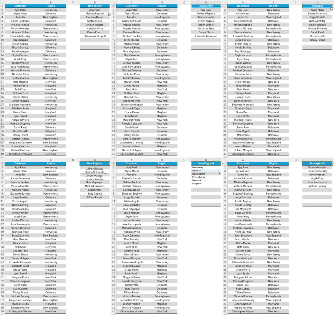
Pro - tip: if you create a validation list for cell D1, you can select other states and the list will update instantly. Check it out…
Adding in Multiple Conditions
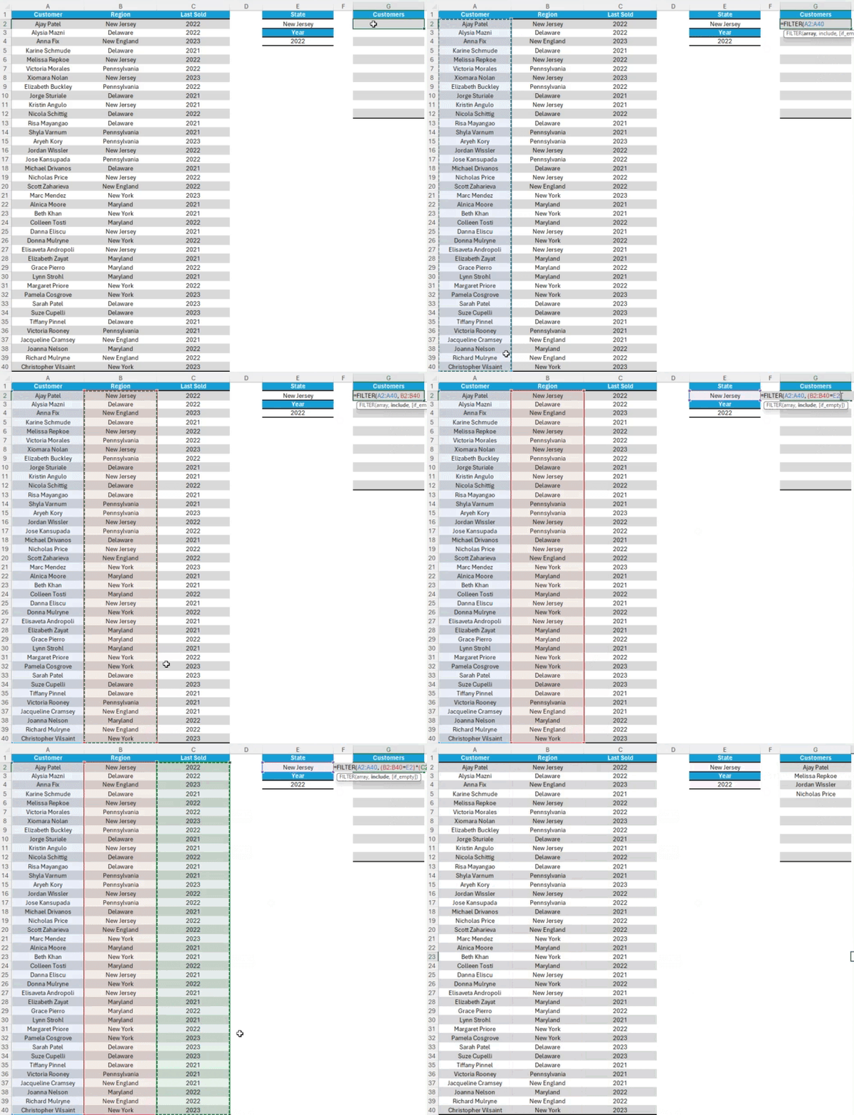
Lets add in an addition condition that we want to filter against. In this case we will include a 3rd column - Last Sold. Now we would like to know which customers in the New Jersey Region made purchases in 2022…
Here is the syntax:
=FILTER(A2:A40, (B2:B40=E2)*(C2:C40=E4))
By the way - you saw that correctly. By using an asterisk between the two conditions you can combine them.
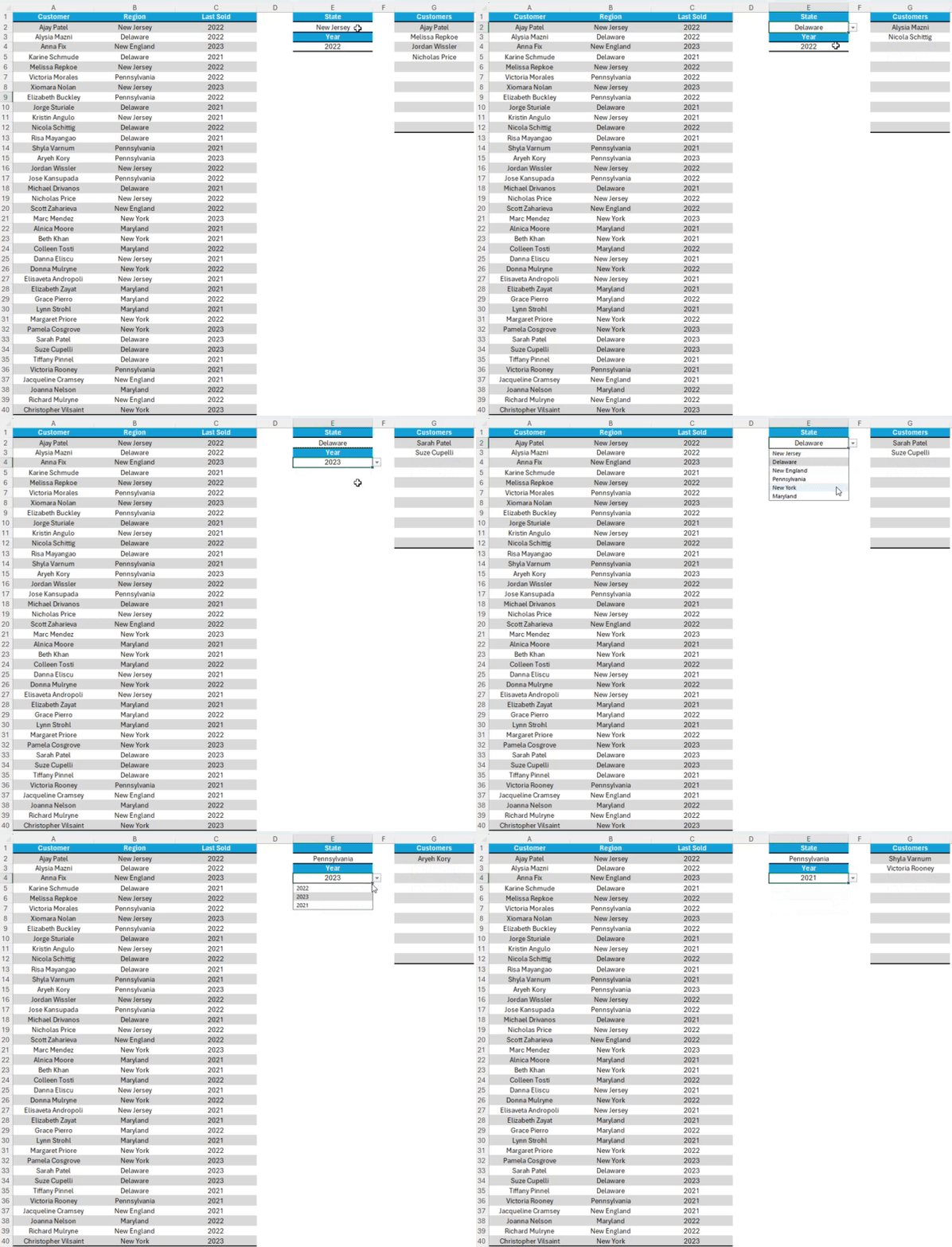
Just like with the last example, if we have data validation for the two input conditions the list will update instantly….
Managing Empty Results
When working with large data sets you are bound to have situations when there is no returnable data. While it is a small thing, an ERROR message isn’t always preferred. Luckily the syntax for =FILTER() allows us to create a message indicating that the data is not present for that particular combination. Here is the updated syntax:
=FILTER(A2:A40, (B2:B40=E2)*(C2:C40=E4), "No Data")
Here it is in application:
Ignoring Certain Results
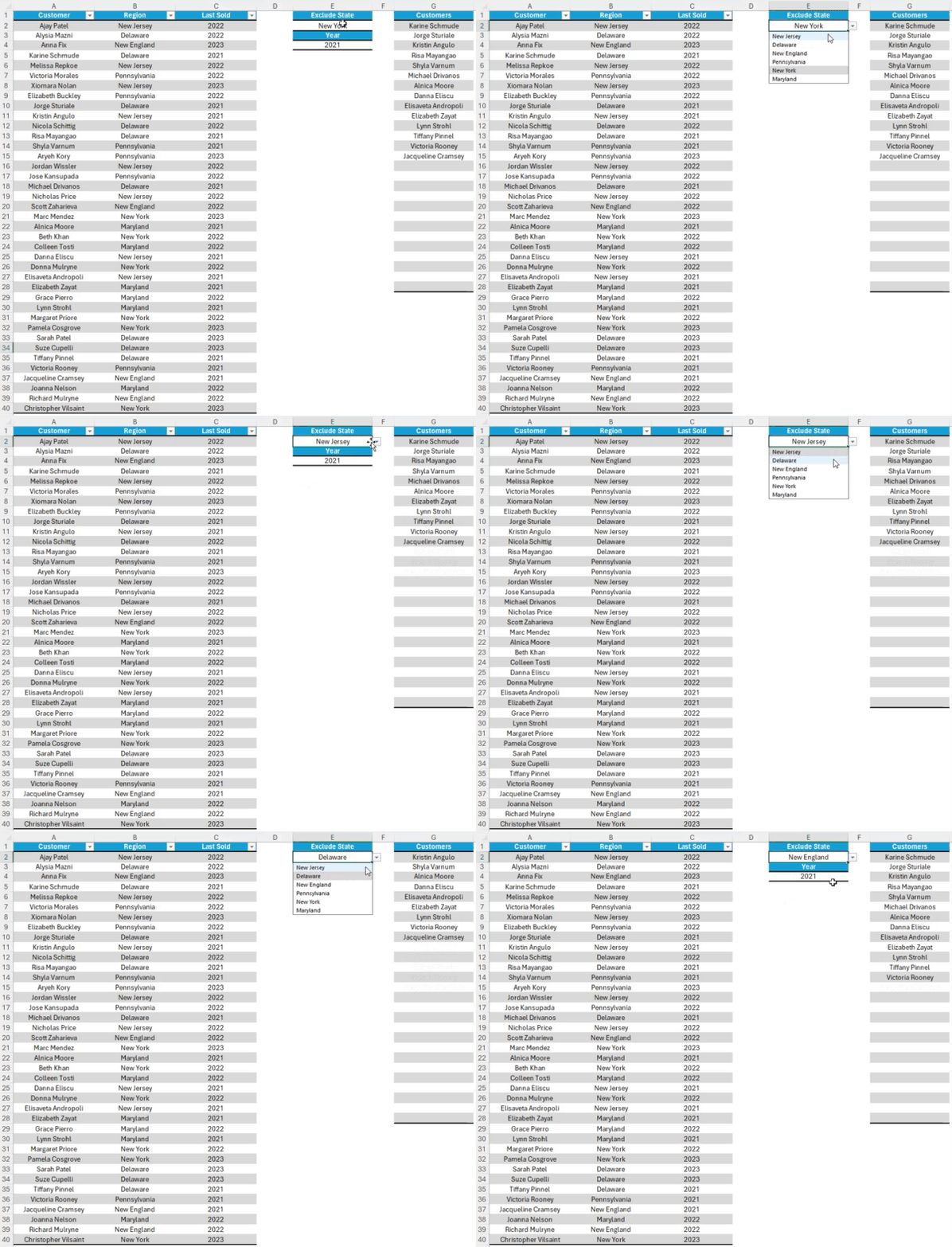
In the previous example we see that there are no customer in NY for 2021. But what if we want to see all the customers in 2021 across all states expect NY? We can adjust the formula and change the equals indicator (“=”) to the does not equal indicator (“<>”). The updated syntax looks like this:
=FILTER(A2:A40, (B2:B40<>E2)*(C2:C40=E4), "No Data")
Now I look at the same data, but instead of being only New York data in 2021, I am looking at all EXCEPT New York in 2021. And because I have a validation menu I can adjust my values as needed.
Thanks for reading this newsletter. The =FILTER() function has certainly made my life a bit easier and now I hope it can do the same for you! Practice does make perfect so be sure to try out the scenarios we covered today. To help you with that I encourage you to make sure you practice what we have covered today. Here is a link to the sample data so that you can follow along:
When you’re ready, there are a few other ways I can help you master Excel:
Do you have any burning questions about Excel that you want answered? Send your question to ajay@theexceldojo.com. I will address it in a future newsletter.
Do you or your organization need a little spreadsheet help? Book a 1 on 1 with me here.
Be sure to follow me on your favorite social media platforms!
Til next time ✌️
-Ajay
The Excel Ninja 🥷
PS - If you found this newsletter informative please share with a friend or two...


